Probability & Bayes Theorem
A Step 1 high-yield lesson connecting the core probability rules and Bayes theorem to diagnostic testing: the 2×2 table, sensitivity/specificity vs. prevalence-dependent PPV/NPV, likelihood ratios, and the SPIN/SNOUT screen-then-confirm logic tested in vignettes.
Why Bayes Runs the Diagnostic Game
Probability quantifies uncertainty, and on Step 1 it lives underneath every diagnostic-testing question. Bayes theorem formalizes how a test result updates the probability of disease: it converts a pre-test probability (in screening, essentially the prevalence) into a post-test probability using the test's performance characteristics.
The board-tested punchline: sensitivity and specificity are intrinsic properties of the test and do not change with prevalence, but the predictive values (PPV/NPV) depend heavily on prevalence in the population being tested. Master the 2×2 table, the four core metrics, and the direction prevalence pushes each value, and most probability items on the exam become plug-and-chug arithmetic rather than conceptual traps.
- AND / independent events → multiply: P(A∩B) = P(A) × P(B)
- OR / mutually exclusive events → add: P(A∪B) = P(A) + P(B)
- General OR (events can overlap): P(A) + P(B) − P(A∩B)
- Conditional probability: P(A|B) = P(A∩B) / P(B)
- Bayes theorem: P(A|B) = [ P(B|A) × P(A) ] / P(B)
- Clinical Bayes: post-test probability = pre-test probability updated by the test result
- Odds form (fast for LRs): post-test odds = pre-test odds × likelihood ratio
- Convert as needed: odds = P / (1 − P); P = odds / (1 + odds)

The 2×2 Table: Four Metrics + Likelihood Ratios
| Metric | Formula | Answers | Prevalence-dependent? |
|---|---|---|---|
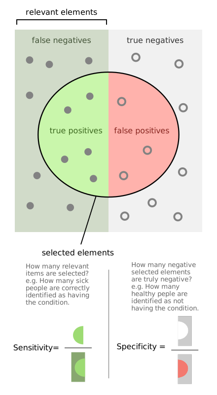
| Sensitivity | TP/(TP+FN) | Detects disease when present | No (intrinsic) |
| Specificity | TN/(TN+FP) | Excludes disease when absent | No (intrinsic) |
| PPV | TP/(TP+FP) | P(disease if test +) | Yes — ↑ with prevalence |
| NPV | TN/(TN+FN) | P(no disease if test −) | Yes — ↓ with prevalence |
| LR+ | Sens/(1−Spec) | How much a + result raises odds | No |
| LR− | (1−Sens)/Spec | How much a − result lowers odds | No |
Vignette: A new screening test for a disease with prevalence 1/1000 has 99% sensitivity and 95% specificity. A patient screens positive. What is the probability she truly has the disease?
Work the 2×2 for 100,000 screened:
- Diseased = 100 → TP = 99, FN = 1
- Well = 99,900 → TN = 94,905, FP = 4,995
- PPV = 99 / (99 + 4,995) ≈ 1.9%
Teaching point: Even a near-perfect test gives a dismally low PPV when prevalence is low — the huge well population generates far more false positives than the tiny diseased pool generates true positives.
Next best step: Do not treat on a single positive screen; confirm with a more specific test first. This is the whole rationale for screen-then-confirm algorithms.
- SP-P-IN — SPecific test, when Positive, rules IN disease (few false positives).
- SN-N-OUT — SeNsitive test, when Negative, rules OUT disease (few false negatives).
- Prevalence & predictive values move oppositely: as prevalence rises, PPV rises and NPV falls.
- Screening = Sensitive first (catch everyone, tolerate false positives); Confirming = Specific second (avoid mislabeling the healthy).
- Sensitivity and specificity are fixed test properties — they do not change when prevalence changes (classic distractor).
- PPV ↑ and NPV ↓ as prevalence ↑; low-prevalence settings make a positive result more likely to be false → low PPV.
- In screening, pre-test probability ≈ prevalence of the population.
- LR+ = Sens/(1−Spec) (ratio of true-positive rate to false-positive rate); LR− = (1−Sens)/Spec.
- LRs are prevalence-independent and let you Bayes-update quickly: post-test odds = pre-test odds × LR.
- Rule of thumb: LR+ >10 or LR− <0.1 produces large probability shifts; LR near 1 barely moves probability.
Vignette: An asymptomatic adult undergoes HIV testing. The initial 4th-generation antigen/antibody immunoassay (highly sensitive) is reactive. What is the next best step?
Answer / next step: Proceed to the HIV-1/HIV-2 antibody differentiation assay (highly specific) to confirm — not repeat the same screen, and not start therapy on a single reactive screen. (If the differentiation assay is negative or indeterminate, an HIV-1 RNA/NAT resolves the discordance.)
Why this order tests Bayes: The sensitive test is deployed first to minimize false negatives (rule out / SNOUT), accepting some false positives. The specific confirmatory test then minimizes false positives (rule in / SPIN) before a diagnosis is assigned. Each step raises post-test probability — sequential Bayesian updating in clinical form.
Practice Biostatistics now
Board-style questions, spaced-repetition flashcards, and a Socratic AI tutor — free to start.