Evidence-Based Medicine Principles
A boards-focused EBM lesson covering the exam's four core tasks — choosing study designs/statistical tests, interpreting sensitivity/specificity/PPV, computing RR/OR/ARR/NNT, and identifying bias — anchored in the 2×2 table with next-best-step reasoning.
What the boards actually test
Evidence-based medicine (EBM) integrates the best research evidence, clinical expertise, and patient values. Boards rarely ask for definitions — they test the mechanics: appraising study design, interpreting test performance, quantifying treatment effect, and spotting bias. Frame the clinical question with PICO (Patient, Intervention, Comparison, Outcome).
Know the hierarchy of evidence: systematic review / meta-analysis of RCTs > single RCT > cohort > case-control > cross-sectional > case series/report > expert opinion. Randomization is the single most powerful tool because it balances known and unknown confounders — nothing else does.
On exam day almost every EBM item is one of four flavors:
- Pick the study design or statistical test.
- Compute or interpret sensitivity / specificity / PPV / NPV.
- Compute RR / OR / ARR / NNT.
- Name the bias and how to fix it.
Master the 2×2 table and a handful of formulas and you own this topic.
Build the 2×2 (disease across the top, test result down the side): TP, FP, FN, TN.
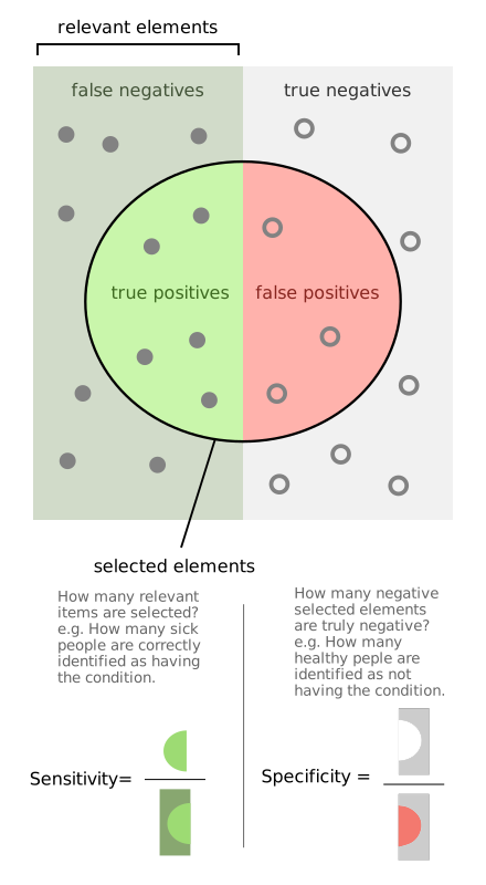
- Sensitivity = TP/(TP+FN) — detects disease. High Sens, a Negative rules out (SnNout)
- Specificity = TN/(TN+FP). High Spec, a Positive rules in (SpPin)
- Sensitivity & specificity are intrinsic to the test — they do NOT change with prevalence
- PPV = TP/(TP+FP) — rises with prevalence
- NPV = TN/(TN+FN) — falls with prevalence
- Low-prevalence screening → many false positives → low PPV (classic tested point)
- LR+ = Sens/(1−Spec); LR− = (1−Sens)/Spec. LR+ >10 or LR− <0.1 = strong test
- Lower the cutoff → ↑sensitivity (fewer FN, good screening test); raise the cutoff → ↑specificity (fewer FP, good confirmatory test)
Study designs at a glance
| Design | Direction | Measure | Best for |
|---|---|---|---|
| RCT | Prospective, randomized | RR / HR | Causation; gold standard for therapy |
| Cohort | Exposure → outcome | Relative Risk (RR) | Incidence; rare exposures; multiple outcomes |
| Case-control | Outcome → exposure (retrospective) | Odds Ratio (OR) | Rare diseases; cheap, fast |
| Cross-sectional | Snapshot in time | Prevalence, OR | "What's happening now"; prevalence |
| Meta-analysis | Pools prior studies | Pooled effect | ↑ statistical power; top of hierarchy |
Vignette: A company markets an HIV antibody screen with 99.9% sensitivity and 99.5% specificity. Deployed to low-risk blood donors (prevalence ≈ 1/10,000), the lab is flooded with positive results, yet nearly all flagged donors are uninfected on confirmatory testing.
Why? In a low-prevalence population, even a highly specific test yields a low PPV — false positives vastly outnumber true positives (here PPV ≈ 2%). Note the test's sensitivity and specificity are unchanged; only PPV shifted, driven by prevalence.
Next best step: Confirm every reactive screen with a confirmatory assay (HIV-1/2 antibody differentiation immunoassay) before disclosing a diagnosis. Never act on a single positive screening test in a low-prevalence setting.
Exam trap: If asked which parameter changed when the same test moves from a high-risk clinic to general screening, the answer is PPV (↓) and NPV (↑) — not sensitivity or specificity.
- Relative Risk (RR) = risk_exposed / risk_unexposed (cohort/RCT). RR =1 no effect, >1 harm, <1 protective
- Odds Ratio (OR) = (a×d)/(b×c) (case-control); ≈ RR when disease is rare
- Absolute Risk Reduction (ARR) = risk_control − risk_treated
- Relative Risk Reduction (RRR) = 1 − RR = ARR / risk_control
- Number Needed to Treat (NNT) = 1/ARR (round up); NNH = 1/absolute risk increase
- Hazard Ratio (HR) = relative event rate over time (Cox/survival analysis)
- Attributable risk % (in exposed) = (RR − 1)/RR
Confidence intervals: a ratio (RR/OR/HR) whose 95% CI crosses 1, or a difference of means whose CI crosses 0, is NOT statistically significant. Narrower CI = more precision (larger n).
High-yield biases and their fixes
| Bias | Classic scenario | Fix |
|---|---|---|
| Selection (Berkson) | Hospital-based controls not representative | Population-based controls |
| Recall | Cases recall exposures better (case-control) | Prospective design; use records |
| Lead-time | Screening detects disease earlier → apparent "longer survival," same death date | Compare mortality, not survival time |
| Length-time | Screening over-catches indolent/slow tumors | Randomized screening trial |
| Confounding | Coffee–cancer link actually driven by smoking | Randomize, restrict, match, stratify, regression |
| Hawthorne | Subjects change behavior when observed | Control group |
| Observer/measurement | Assessor knows the assignment | Blinding; objective criteria |
Vignette: A cohort finds coffee drinkers have 2× the rate of lung cancer. After adjusting for cigarette smoking, the association vanishes (RR → 1.0). In a separate analysis, an occupational carcinogen's effect on lung cancer is much larger in smokers than non-smokers, and this stratum difference persists after adjustment.
First finding = confounding. Smoking is associated with both coffee and lung cancer and lies on no causal path from coffee → cancer; adjustment removes the spurious link.
Second finding = effect modification (interaction). The true effect genuinely differs by stratum — report stratum-specific estimates; do NOT "adjust it away" or report a single pooled number.
Next best step for a confounder: control it — randomization, restriction, matching (design), or stratification / multivariable regression (analysis). Randomization handles unknown confounders too.
- SpPin — a highly Specific test, when Positive, rules in.
- SnNout — a highly Sensitive test, when Negative, rules out.
- Type I error (α) = false positive — you "cry wolf" / convict the innocent — reject a true null. Its rate is the significance level α (typically 0.05).
- Type II error (β) = false negative — you "miss the wolf." Power = 1 − β, raised by larger sample size, larger effect size, and higher α.
- Picking the test: compare means of 2 groups → t-test; 3+ groups → ANOVA; categorical/proportions → Chi-square ("Chi = chategorical").
Practice Research Methods now
Board-style questions, spaced-repetition flashcards, and a Socratic AI tutor — free to start.