Descriptive Statistics & Distributions
A board-focused walkthrough of central tendency, dispersion, and the normal distribution's 68-95-99.7 rule — showing how skew and outliers shift the mean versus median, plus the SD-vs-SEM trap and the z-score-to-percentile conversions Step 1 loves to test.
Descriptive statistics summarize a dataset with two things: a measure of central tendency (where the middle sits) and a measure of dispersion (how spread out the data are). On Step 1 the tested skill is choosing the correct measure for a given distribution and predicting how an outlier or skew shifts the mean relative to the median. Central tendency = mean, median, mode. Dispersion = range, IQR, variance, standard deviation (SD), and — for a sampling distribution — the standard error of the mean (SEM). The distribution's shape (normal vs skewed vs bimodal) decides which summary is trustworthy and how the mean, median, and mode line up. Master three moves: (1) read the shape, (2) rank mean/median/mode, (3) convert '# of SDs from the mean' into a percentile.
Central tendency
- Mean = arithmetic average; most affected by outliers/skew (dragged toward extremes).
- Median = middle value (50th percentile); robust to outliers → best for skewed data.
- Mode = most frequent value; the only measure usable for nominal (categorical) data; a set can be bimodal (two modes).
Dispersion
- Range = max − min; very sensitive to outliers.
- Variance (σ²) = average squared deviation from the mean.
- SD = √variance; average spread in the original units.
- IQR = Q3 − Q1 (middle 50%); robust, pairs with the median (boxplot).
- SEM = SD/√n → precision of the sample mean; < SD (for n > 1) and shrinks as n grows.
Normal (Gaussian) distribution — the 68-95-99.7 empirical rule
- Symmetric, bell-shaped; mean = median = mode all at the center.
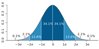
- ±1 SD ≈ 68% of the data (leaves ~16% in each tail).
- ±2 SD ≈ 95% (precisely ±1.96 SD = exactly 95%; leaves ~2.5% per tail).
- ±3 SD ≈ 99.7%.
- Worked example: serum Na⁺ normally distributed, mean 140, SD 3 → 95% of people fall ~134–146 (140 ± 2×3).
- z-score = (value − mean)/SD = how many SDs from the mean. Convert a z-score into a percentile using the rule above.
| Distribution | Shape | Mean · Median · Mode | Best central measure |
|---|---|---|---|
| Normal | Symmetric bell | Mean = Median = Mode | Mean |
| Positive (right) skew | Long tail to the right | Mean > Median > Mode | Median |
| Negative (left) skew | Long tail to the left | Mean < Median < Mode | Median |
| Bimodal | Two peaks | Two modes | Inspect / report both |
Vignette: A study reports hospital length of stay (LOS) for 200 patients. Most stay 3–5 days, but a handful of ICU patients stay 60+ days. The mean LOS is 8 days, but the median is 4 days.
- Interpretation: the long-stay outliers create a positive (right) skew; the mean is pulled toward the high tail → mean > median.
- Which to report (next best step): use the median (4 days) — robust to outliers and more representative of the typical patient.
- Pattern recognition: LOS, income, hospital charges, and time-to-event data are classically right-skewed → default to the median.

SD vs SEM vs 95% CI — a classic Step 1 trap
- SD describes spread of individual data points in one sample. Does not shrink systematically with sample size.
- SEM = SD/√n describes precision of the sample mean (spread of the sampling distribution). Shrinks as n increases. Authors sometimes report SEM (smaller) to make data look tighter than SD would.
- 95% CI ≈ mean ± 1.96 × SEM → range expected to contain the true population mean 95% of the time; wider CI = less precise.
- If a 95% CI crosses the null → not statistically significant (null = 0 for a difference in means, 1 for an RR/OR).
Vignette: A 6-year-old girl's height is exactly 2 SD below the population mean on a normally distributed growth chart. What percentile — and what does it suggest?
- ±2 SD spans the central 95%, leaving 5% split between the tails → 2.5% in each tail.
- A value 2 SD below the mean (z = −2) sits at roughly the 2.5th percentile.
- ±1 SD → ~16th and ~84th percentiles (68% central, 16% per tail).
- Clinical link: short stature = height < −2 SD (≈ <2.5th percentile) or < 3rd percentile for age/sex → warrants evaluation.
- Key move: convert z-score → percentile with 68-95-99.7.
- "The mean is MEAN to outliers" — the mean is dragged toward extreme values; the median stays robust. So for skewed data (LOS, income, charges), report the median.
- "The mean chases the tail" — in any skew, the mean is pulled toward the long tail. Right (positive) skew → tail and mean on the high side → Mean > Median > Mode.
- 68-95-99.7 — the empirical rule for ±1, ±2, ±3 SD in a normal distribution. Locks in that ±2 SD ≈ 95% (and ~2.5% per tail).
Practice Biostatistics now
Board-style questions, spaced-repetition flashcards, and a Socratic AI tutor — free to start.