Correlation & Regression
A high-yield Step 1 lesson on correlation vs. regression: interpreting the correlation coefficient r, the causation trap, r² as variance explained, and choosing linear vs. logistic regression. Built around the exact interpretation errors the boards test.
Correlation and regression both describe the relationship between two continuous variables, but they answer different questions. Correlation quantifies the strength and direction of a linear association with a single number, the correlation coefficient (r). Regression goes further: it fits a best-fit line and produces a predictive equation, letting you estimate an outcome (dependent variable, Y) from a predictor (independent variable, X). On Step 1 the questions are almost never computational — they test interpretation. The three classic traps: confusing r with r², assuming a correlation proves causation, and forgetting that r captures only linear relationships. The scatterplot is the visual companion: the tighter the points hug a straight line, the closer |r| is to 1.
- r (Pearson correlation coefficient) = strength + direction of a linear relationship between two continuous variables
- Range −1 to +1: the sign gives direction, the absolute value gives strength
- r = +1 perfect positive; r = −1 perfect negative; r = 0 no linear correlation
- Correlation ≠ causation — an association may be explained by confounding
- r = 0 excludes only a linear link; a U-shaped/nonlinear relationship can still exist
- r is unitless and unchanged by rescaling units (e.g., cm → inches)
- Outliers can dramatically distort r
- A low p-value means the correlation is statistically significant (unlikely by chance) — NOT that it is strong or causal
- r² (coefficient of determination) = proportion of variance in Y explained by X

Vignette: An investigator plots serum LDL against coronary artery calcium score in 200 adults and finds r = 0.85 (p < 0.001). A colleague concludes that lowering LDL will reduce calcium scores.
- Interpret r: strong positive linear correlation
- The flaw / best response: correlation does not establish causation. This observational association can be confounded (age, smoking, diabetes); only a randomized controlled trial supports causation
- r² = 0.85² ≈ 0.72 → about 72% of the variance in calcium score is explained by LDL; the other ~28% is other factors
- Distractor to avoid: the tiny p-value proves only statistical significance, not causation or clinical importance
Next step in reasoning: to claim causality, design an interventional (RCT) study, not another observational correlation.
| Feature | Correlation | Regression |
|---|---|---|
| Question | How strong / which direction? | Predict Y from X |
| Output | r (−1 to +1) | Line: Y = a + bX |
| Roles of X, Y | Symmetric (interchangeable) | Directional (predictor → outcome) |
| Units | Unitless | Slope b has units (ΔY per ΔX) |
| Causation | No | No (prediction ≠ causation) |
| Variance explained | r² | R² |
| Adjust for confounders? | No | Yes (multiple regression) |
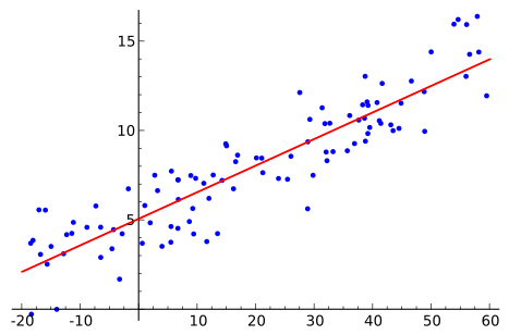
- Linear regression models a continuous outcome: Y = a + bX; slope b = change in Y per 1-unit change in X
- Slope b > 0 positive relationship; b < 0 negative (inverse); b = 0 no relationship
- Intercept a = value of Y when X = 0
- Slope steepness ≠ correlation strength: a steep line can have a weak r and a shallow line a strong r — r reflects scatter about the line, not its slope
- Multiple linear regression = several predictors at once → its main strength is adjusting for confounders
- Logistic regression models a binary/dichotomous outcome (disease yes/no, dead/alive); effect is reported as an odds ratio
- Converting r → r²: always square r. r = 0.6 → r² = 0.36 → 36% of variance explained (NOT 60%)
- After squaring, r² is always ≥ 0; a negative r gives the same r² as its positive twin
Vignette: A study reports that weekly hours of exercise and resting heart rate have r = −0.6.
- Direction: negative — more exercise is associated with a lower resting HR (inverse relationship)
- Strength: moderate
- Variance explained: r² = (−0.6)² = 0.36 → 36% of the variability in resting HR is explained by exercise hours
- Classic distractor: "r = −0.6 means 60% of variance is explained" — wrong; you must square r
- The negative sign reflects a real inverse association but has no effect on the magnitude of r²
Take-home: whenever a question gives you r and asks about variance/variability explained, square it first.
| Feature | Linear regression | Logistic regression |
|---|---|---|
| Outcome (Y) | Continuous (BP, weight, LDL) | Binary (disease: yes/no) |
| Equation | Y = a + bX | logit(p) = a + bX |
| Effect measure | Slope (ΔY per 1-unit ↑ in X) | Odds ratio (e^b) |
| Example | Predict blood pressure from BMI | Predict MI (yes/no) from LDL |
| Board buzzword | "for each 1-unit ↑ in X, Y changes by b" | "odds ratio," "dichotomous outcome" |
Practice Biostatistics now
Board-style questions, spaced-repetition flashcards, and a Socratic AI tutor — free to start.